rasterDT uses the fast indexing, aggregation, and assignment operations provided by data.table to power speedy alternatives to several raster package functions. The functions that it provides are between 5 and 25 times faster than the raster package functions that they replace.
Installation
Use devtools to install the current version of rasterDT:
devtools::install_github("JoshOBrien/rasterDT")Usage
rasterDT functions take the same arguments as their raster package equivalents and are designed (with a very few exceptions) to return the same values. Like their raster equivalents, they work with rasters that are too large to hold in memory and (with the exception of fasterizeDT) on RasterLayer, RasterStack and RasterBrick objects.
Because this package leans so heavily on data.table, tabular results are returned as data.tables instead of data.frames. If you would prefer a data.frame, just wrap a data.table object in a call to data.frame().
Performance
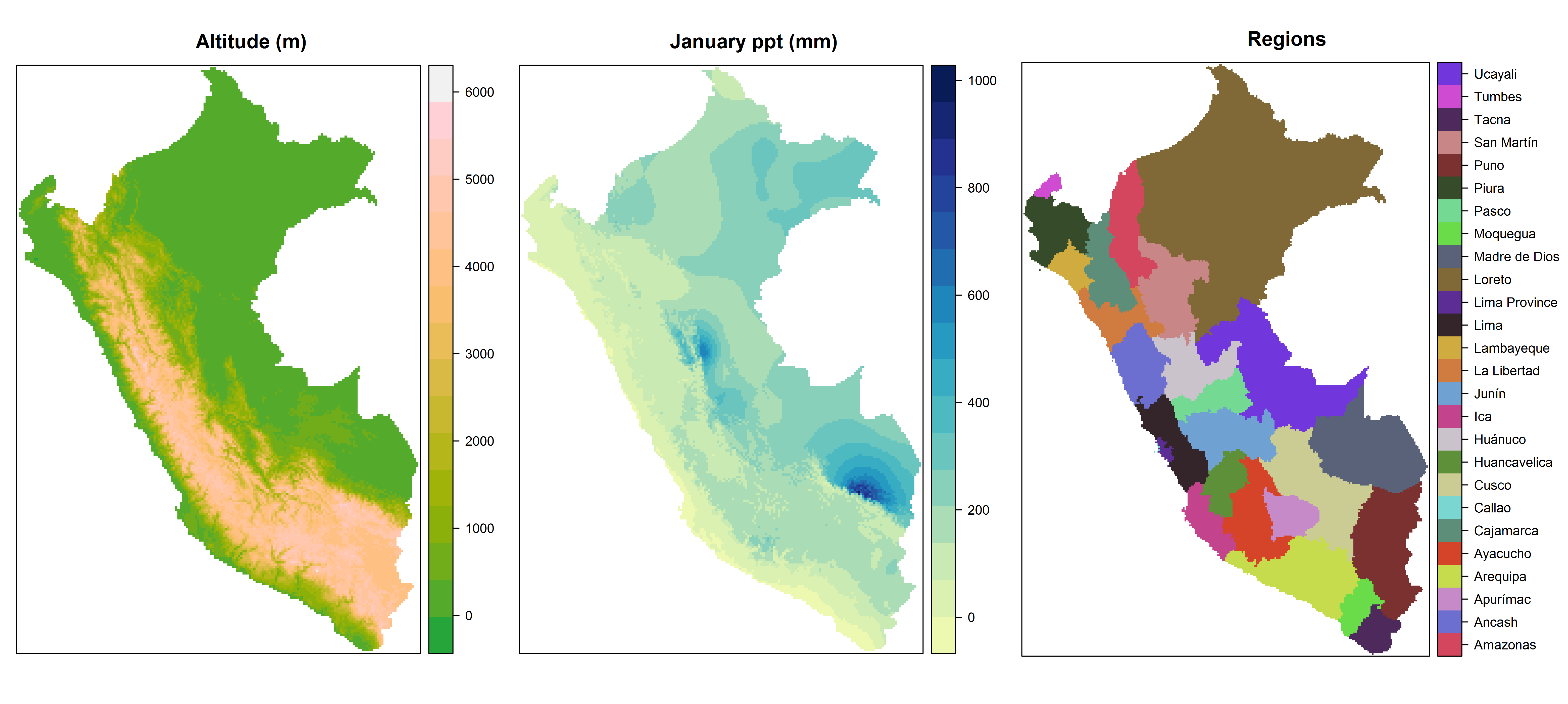
Let’s compare the speed of rasterDT functions with their raster package equivalents. To do so using realistic data, first use raster::getData() to download and prepare three raster layers which display the altitude, January precipitation, and political regions of Peru at a resolution of one half arc minute.
(PLEASE NOTE: running the (fully reproducible) code below will download several raster files into the working directory of your current R session.)
library(rasterDT)
library(rasterVis)
library(microbenchmark)

## Altitude in m
altitude <- getData("alt", country = "PER", res = 0.5)
altitude <- crop(altitude, extent(altitude) - c(0, 0.2))

## Political subdivisions (categorical)
regions_shp <- getData("GADM", country = "PER", level = 1)
regions <- fasterizeDT(regions_shp, altitude, field = "NAME_1")

## January precipitation in mm
precip <- getData("worldclim", var = "prec", res = 0.5,
                  lon = -75, lat = -15)
precip1 <- crop(precip[[1]], regions)
precip1 <- mask(precip1, regions)
The three resulting rasters are displayed (using plotting calls not shown here) in the figure below:
Next, to estimate the degree of speedup gained by using each rasterDT function relative to its raster package equivalent, we benchmark pairs of functions, executing equivalent calls 5 times and comparing the average timings:
freqDT() vs. freq(): ~6x speedup
microbenchmark(freqDT = freqDT(altitude),
               freq   = freq(altitude),
               times = 5)
## Unit: milliseconds
##    expr       min        lq      mean    median        uq       max neval cld
##  freqDT  358.1587  373.9958  402.0715  375.5939  404.4736  498.1357     5  a
##    freq 2481.5614 2570.1578 2583.9395 2605.2673 2611.1084 2651.6024     5   b

out_freqDT <- freqDT(altitude)
out_freq <- freq(altitude)
crosstabDT() vs crosstab(): ~6x speedup
microbenchmark(crosstabDT = crosstabDT(altitude, regions),
               crosstab   = crosstab(altitude, regions),
               times = 5)
## Unit: milliseconds
##        expr       min        lq     mean    median       uq      max neval cld
##  crosstabDT  934.0795  934.6892 1028.893  979.0466 1147.490 1149.160     5  a
##    crosstab 6274.8551 6430.1598 6439.387 6454.1255 6509.927 6527.869     5   b

out_crosstabDT <- crosstabDT(altitude, regions)
out_crosstab <- crosstab(altitude, regions)
zonalDT() vs zonal(): ~11x speedup
microbenchmark(zonalDT = zonalDT(altitude, regions, min),
               zonal   = zonal(altitude, regions, min),
               times = 5)
## Unit: milliseconds
##     expr       min        lq      mean    median        uq       max neval cld
##  zonalDT  200.5657  204.6846  206.6882  207.9012  209.0513  211.2381     5  a
##    zonal 2195.7178 2199.3366 2242.2448 2219.9958 2266.3005 2329.8735     5   b

out_zonalDT <- zonalDT(altitude, regions, min)
out_zonal <- zonal(altitude, regions, min)
subsDT() vs subs(): ~23x speedup
dict <- zonalDT(altitude, regions, min, na.rm = TRUE)
microbenchmark(subsDT = subsDT(regions, dict),
               subs   = subs(regions, dict),
               times = 5)
## Unit: milliseconds
##    expr       min        lq      mean    median        uq       max neval cld
##  subsDT  250.4851  254.4848  356.3356  259.0266  293.7392  723.9421     5  a
##    subs 8077.3643 8086.8702 8167.4095 8184.9779 8186.2390 8301.5961     5   b

out_subsDT <- subsDT(regions, dict)
out_subs <- subs(regions, dict)
fasterizeDT() vs rasterize(): ~25x speedup
## rasterize()'s field= argument can handle factor but not character vectors
regions_shp$NAME_FAC <- factor(regions_shp$NAME_1)
microbenchmark(fasterizeDT = fasterizeDT(regions_shp, altitude, field = "NAME_FAC"),
               rasterize   = rasterize(regions_shp, altitude, field = "NAME_FAC"),
               times = 5)
## Unit: milliseconds
##         expr        min         lq      mean     median         uq       max
##  fasterizeDT   48.09048   49.00721  107.8917   51.78699   52.29528  338.2786
##    rasterize 2693.34767 2734.66681 2748.1537 2763.89009 2771.21738 2777.6464

out_fasterizeDT <- fasterizeDT(regions_shp, altitude, field = "NAME_FAC")
out_rasterize   <- rasterize(regions_shp, altitude, field = "NAME_FAC")